November 2001

The Order 1 Soil Survey

Soil Management in Site-Specific Agriculture

Update on Order 1 Soil Surveying: Issue 1 of 3

G.K. Blumhoff, SSMC Information Systems Manager

In the June 2001 SSMC newsletter, Keith Morris provided the framework, information abut, and potential of the Order 1 Soil Survey. As an extension of his work, Purdue faculty and Natural Resource Conservation Service (NRCS) soil scientists decided to begin the second phase of the Order 1 soil survey project. This was conducted in an effort to examine current data collection methods and test the usefulness of data sets such as multispectral images, high resolution topography information, and other associated Geographic Information System (GIS) data layers. In addition, we decided incorporate DGPS using a handheld device, and software capable of multiple GIS layer display, including image data. More important, this second phase of soil mapping focused on an applied approach rather than an academic approach to mapping soil characteristics. One of the main goals was to determine if Global Positioning System (GPS) equipment, remote sensing, and other GIS data layers would be useful given the type of data used and the ability to display them in real-time in the field. This article focuses on the data collection process that occurred in the field.

An important question was: How valuable are supplemental data sets such as remote sensing and topography for improving soil map production efficiency and for maintaining data quality?

The second phase of soil mapping was performed on about 110 acres of farmland cropped in a no-till corn-soybean rotation at the Davis Purdue Ag Center (DPAC) in Randolph County, east central Indiana. On average, two soil scientists and one spatial information specialist were present during the mapping period (6 days in the field). Standard mapping techniques were used in addition to transect sampling to delineate soil types. Basic tools included a Munsell color chart, acid bottle, soil probe, and an experienced pair of eyes. Flagging was used to delineate between different soil units, help guide the direction of sampling, and for recording the density of soil cores collected.

It is important to recognize the valuable skills required to perform this mapping provided by Purdue faculty, Gary Steinhardt and Steve Hawkins and NRCS staff, Gary Struben and Bill Hosteter, trained in the science of soil mapping. Soil interpretation can be dirty and difficult, especially in adverse conditions. As an example, the mapping took place during November and occurred just after harvest. Thus, much of the soil mapping occurred with high levels of crop residue present. This greatly affected an observer's ability to visualize the landscape, topography, and soil color changes which are all helpful tools used in the classification process. The first phase of the Order 1 had been conducted under near-zero crop residue conditions, thus minimizing its effect on topography, soil color, and the landscape.

Let us consider the site-specific application and spatial technology aspects of the mapping process. Several spatial technologies were utilized during the second Order 1 soil survey, they included GPS, GIS, and remote sensing data. GPS equipment included a DGPS receiver, handheld computer, and software capable of multiple GIS layer display. All data sets used and created were referenced with UTM coordinates. Typical file formats used were ".shp, .sid, and .jpeg". Available datasets used included: a digitized Order 2 soil survey, and an IKONOS panchromatic image obtained on 1 June 2001 (bare soil 2001), ATLAS Thermal infrared obtained on 5 May 1999 (bare soil 1998), 6" topographic intervals (laser guided leveling), field boundaries, and existing tile maps. It is important to note that the thermal data were used in response to field management issues that occurred in 2000 and 2001 that masked some of the underlying soil conditions present in one of the fields in the project. Currently, there are no approved guidelines for producing estimated soil type boundaries before field entry based on the data sets listed. Therefore, no attempt was made to predict soil boundaries before the field mapping process took place.

Mapping procedures included the collection of polygons, polylines, and points for every flag and soil boundary delineated. Flag locations were referenced for location tagging, to record the density of samples collected, and to provide a safeguard against polyline or polygon data loss. During the mapping process, soil boundaries were mapped with a 10 foot location tolerance. This became important where two soil type boundaries converged. Soil type boundaries were combined or connected when their differences could not be differentiated at distances less than 10 feet apart. Finally, to reduce bias associated with GPS guidance and GIS data layer field display, the soil scientists performed their standard soil mapping techniques in addition to the use of the spatial interaction. GPS navigation was performed along side the soil scientists as a quality check, decision support or "tie breaker", validation, and for verification.

Figure 1 shows the data sets used in the soil mapping process. The digital image map includes a geo-referenced .jpeg IKONOS bare soil image, 6" interpolated contour lines, and existing tile history available for the three labeled fields. Fields R and V shown on the map were planted to soybeans in 2001. Field W was half in corn and half in soybeans. This was both critical and provided challenges since all mapping was performed within days of harvest. Figure 2 shows the ATLAS thermal bare soil data collected in 1999 for field W. This was used to reduce the “noise” from past management practices (i.e. plot research, variable crop-type residue, and varying tillage practices) which are visible in field W in Fig. 1. Notice that the darker areas in the IKONOS data (Fig. 1) are areas where wet soil conditions are common. The opposite can be viewed in Fig. 2 where the darker areas represent dryer soil conditions. This sometimes caused a problem when toggling GIS layers on/off and navigating between fields.

After the three fields were completely mapped and flagged, the GPS data was downloaded and prepared for printing and combined into one file for easy display on the GPS handheld computer,whish was the final step in the data collection process. The maps were reviewed and directed points were delineated at locations where additional soil cores would be collected. This was performed to check accuracy, smooth irregular patterns, or fine-tune the map results to include any smaller soil units. Figure 3 and Figure 4 are soil map displays of the three fields before mapping (Order 2) and after (Order 1). Notice that some of the soil series in Fig. 4 are the same but display a different color. The Order 1 and 2 soil surveys maintain different requirements for soil descriptions (National Soil Survey Handbook). The Order 2 normaly includes soil name and soil unit (Condit silt loam, Condit). The Order 1 includes the soil unit and name, great group and subgroup (Condit silt loam, Condit, Typic Epiaqualfs). Thus, the Order 1 survey showed one additional soil unit along with six different soil types classified to the great group-subgroup level.

A brief glance at the Order 1 versus Order 2 reveals striking differences in map detail and the number of soil units delineated. Also, there are several cases where soil types were split apart rather than lumped together as in the Order 2. The Order 1 data adheres to the remote sensing and topographic data more closely than does the Order 2. It is important to note that small soil unit polygons (i.e. Condit series in field W) were verified with the use of a hydraulic soil probe to obtain a much deeper and broader soil sample for interpretation.

A few comments on the usefulness of the GPS equipment and spatial data sets may be of value to others interested in using our approach. The added GPS and spatial information allowed us to map at a slightly faster pace than would have otherwise been possible. Under the circumstances, during a portion of the mapping process a drizzle and light rain occurred. We were forced to find efficient ways to map. The GPS and spatial data helped in navigating along the contour lines so the soil scientists could gauge where to start collecting samples. The remote sensing data were useful when minor changes in soil conditions were present. The image data displayed different color tones allowing for navigation to center points or areas of greater contrast, thereby helping the soil scientists calibrate soil observations in soil transitional areas. Other benefits included quality control during periods of the day when fatigue sets in, assistance at locations where slight changes in topography exist, and where heavy crop residue was present. It is important to mention that half of field W was at or near 100% residue cover since corn was harvested only a day prior to mapping. Under these conditions, GPS and spatial data guided and helped pinpoint locations where soil cores would provide the most information.

Interestingly, none of the soil scientists had any prior exposure to spatial data in digital form. Their previous experience was limited to hard copy topographic maps and aerial photography. By the end of the mapping process, the scientists were comfortable with and readily utilized the information to help them in the mapping process. At a minimum, the technology removed error, guesswork, and improved the overall quality of the surveying process.

Please check out upcoming newsletters related to spatial data and the Order 1. This document is the first in a series of three newsletters outlining the processes and comparison of spatial data and the Order 1. Upcoming newsletters will include information on the lab/computer portion of the mapping process (i.e. digitizing, soil map creation, clean up, etc.) and comparisons made between yield data and EC data.

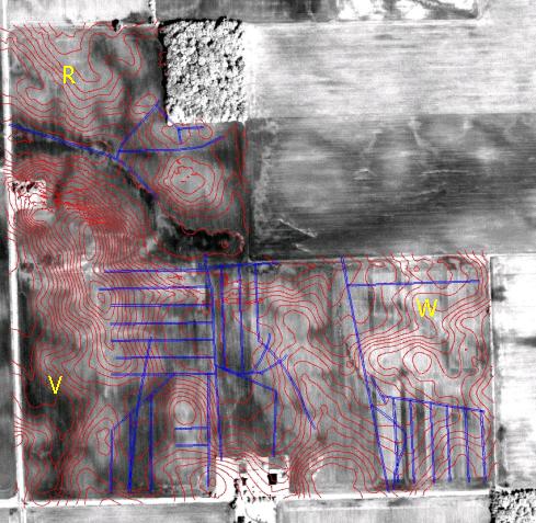
Figure 1. Display of 2001 bare soil IKONOS image data, tile lines, and 6" contours of elevation. Red letters indicate the field id.

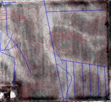
Figure 2. Display includes 1999 bare soil ATLAS thermal image data along with tile lines and 6" contour elevation for field W.

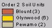
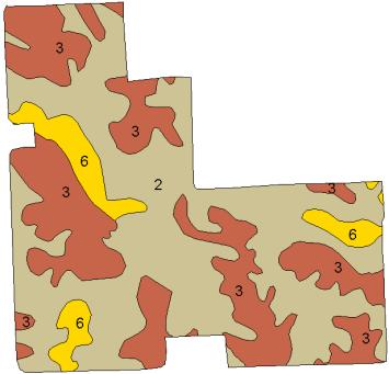
Figure 3. Order 2 soil survey map of fields R, V, and W. Soil series are included on the map.

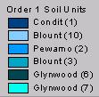
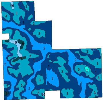
Figure 4. Order 1 soil survey map of fields R, V, and W. Soil series are included on the map.